Condition values in ms excel

Condition values in ms excel

Hi Sik,

That should be found in the formatting option whereby you can set it to either conditional or unconditional.

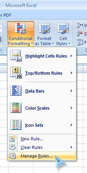
While in excel, go to home then conditional formatting, then manage rules. In the dialog box that will appear state the conditions accordingly, stating what action should be taken so that when the conditions are stated, the colours are applied.

When you are done editing and stating the conditions, click ok and go back and try editing the cells that you have applied the conditions to and see how they work.

For an extensive procedure on how to go about the whole process, please visit the link below:

Download Link

Hope this helps.

___

Regards,

Lee Hung.

Condition values in ms excel

Here is an example of what you want to accomplish. See the table above. To create the table above, you need to use Conditional Formatting in Microsoft Office Excel. First, create the table as shown in the image above. Don’t apply colors on the values under Remarks. The colors will be automatically applied using Conditional Formatting. Once the table is created, click Conditional Formatting under Styles section in Home tab. See image.

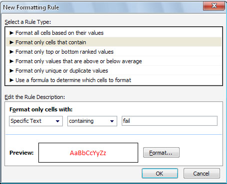
Select New Rule. In New Formatting Rule dialog box under “Select a Rule Type” section, select “Format only cells that contain”. Under “Edit the Rule Description” section, on the first option select Specific Text. On the second option, select “containing”. On the third and last option, enter the text without quotes “pass”. After that, click Format and then select the color green for the font color.

You can also apply a background color on the cell using the Fill tab. Click OK all through out when you are done. See image.

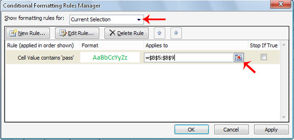
You won’t see any changes yet on the table after this. Next, click Conditional Formatting and then select Manage Rules. See image.

In Conditional Formatting Rules Manager dialog box, select the rule you created. If you don’t see it, select an option in “Show formatting rules for”. Under “Applies to”, click on the small red arrow. After that, select the cells where the values Pass and Fail should appear and then click on the small red arrow again. Click Apply and then OK. See image.

After this, all cells that contain the text “Pass” will have a green color. Again, click Conditional Formatting and then select New Rule. Select “Format only cells that contain”. On the first option, select Specific Text. On the second, select “containing”. On the third option, enter without quotes “fail”. After that, click Format then select the color red for the font color and then click OK all through out.

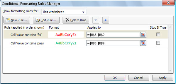
Click Conditional Formatting and then select Manage Rules. Select the rule with the red color. Click on the small red arrow, select the same cells where Pass and Fail should appear, and then click on the small red arrow again. The two rules you created should have the same range of cells. Click Apply and then OK.

After this, you should see the cells containing the text “Fail” in red color.