MS Excel is a vital software program of Office Suite developed by Microsoft. It is spreadsheet software that uses rows and columns to organize, store and calculate data. It generally runs on Windows, macOS, Android, and iOS. You can quickly learn Excel. In Excel, you can do more advanced things as you become better. It is used for both office work and daily life. Excel is mainly used for data analysis, data entry, management, accounting, budgeting, and financial purposes. Excel generally has shortcut keys to speed up the process. Below are the most valuable tricks for data analysis that provide you with the tools to handle most of your Excel data analysis tasks.
1. Vlookup
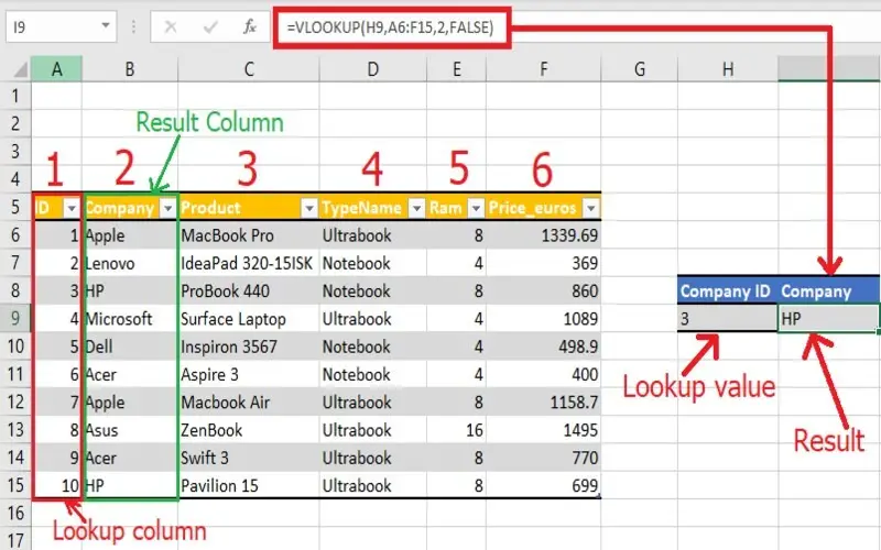
VLOOKUP stands for Vertical Lookup. It is an excellent function for data analysis. This function makes the task easy and quick. It brings back the values either from different spreadsheets or workbooks. You can use VLOOKUP to find things in a table or a range of rows. VLOOKUP consists of four points to build syntax:
- The value you want to look up at is called the lookup value.
- Then, where to look up the value.
- The column number in the range consists of the return value.
- Then, what type of lookup would you like to do, TRUE or FALSE? Use TRUE if you want an approximate match and FALSE if you want an exact match, the return value. Now put the value in the following syntax: =VLOOKUP(lookup value, range of data you want to search for, column index number, range lookup value – either TRUE or FALSE)
2. Concatenate
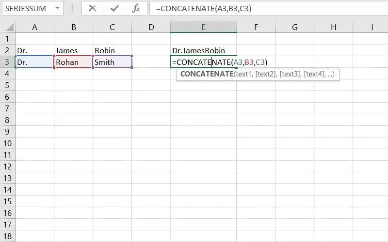
The CONCATENATE word means to join or combine. This function in Excel combines the text, numbers, dates, and other data from different cells into one cell. For example, this function connects the first and last names into full names. Hence, a space is entered for the text2 argument. The Syntax for the CONCATENATE FUNCTION is: =CONCATENATE(text1, text2, text3,…)
3. Xnpv
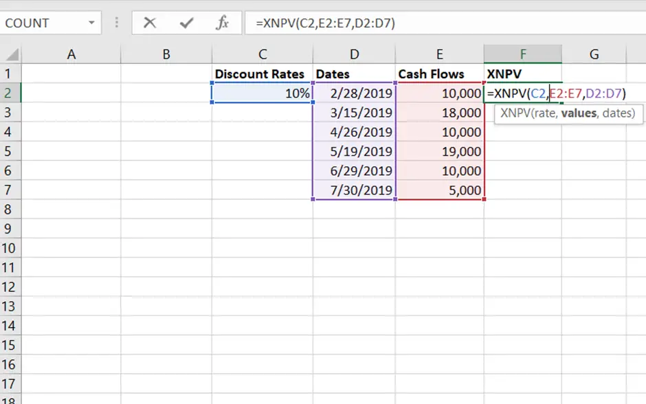
This XNPV function in Excel is used to calculate the net present value of an investment by using a discount rate and a series of cash flows at irregular intervals. Financial department analysts use this function. The formula for the XNPV function is: =XNPV(rates, cash flow, dates of cash flow)
4. Xirr
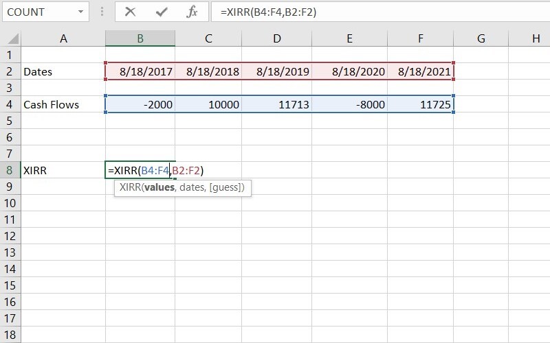
It stands for Extended Internal Rate of Return. It is used to calculate returns on investment for a series of cash flows that may not be periodic. It helps in deciding the value of an investment. Using the XIRR Excel function, we learned that unevenly timed cash flow could be accurately modeled. The formula for the XIRR function is: =XIRR(values,dates,[guess]) Guess – A number that you guess is close to the XIRR.
5. Len
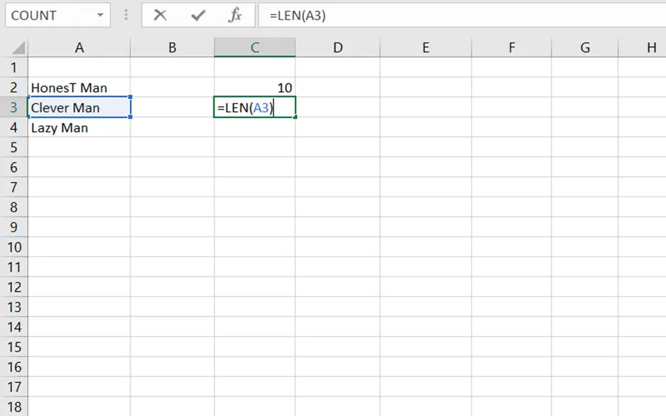
The function LEN is also called the LENGTH Function. This function calculates the length of a text in an Excel cell or a range of cells. You can use the LEN function for data validation – to ensure that a set number of characters are entered into a cell and data cleaning – to identify cells containing a fixed number of characters and then use those details to clean your data. The formula for the LEN function is: =LEN(cell value)
6. Trim
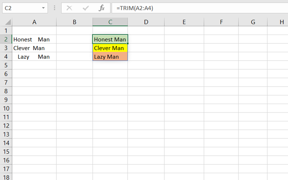
The TRIM function in Excel removes extra spaces or characters from text except for single spaces between words. This function is used to normalize all spacing. This function is convenient and beneficial when we have copied text from different sources and want to remove extra spacing from the text. The formula for the TRIM function is: =TRIM(cell value/text)
7. Index-match
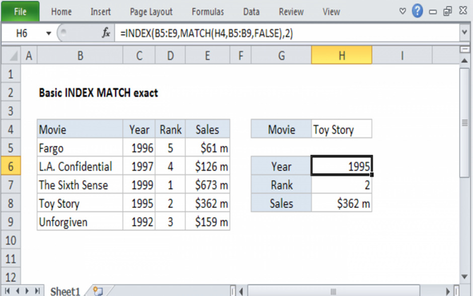
This INDEX-MATCH combination function handles horizontal and vertical data very quickly, and it can look up and return the deals and discounts of a cell in a table. You can use the INDEX function to get the values from an entire row or column. At the same time, the MATCH function is used to get the position of the whole row or column. It is beneficial for finding a value in a column to the left. If you get stuck in using VLOOKUP to get back from a column towards the right, then you can use the INDEX-MATCH function instead of VLOOKUP; it will consider the lookup and return column. The formula for the INDEX-MATCH function is: =INDEX(reference table [row], [column], [MATCH(SearchKey,Range,SearchType)]) The search type is 0 or 1. 0 is used to find the exact value when the range is unsorted. One is used to seeing the most significant value, less than or equal to the search key when the content is sorted in ascending order; if the content is in descending order, you can use-1.
8. Xlookup
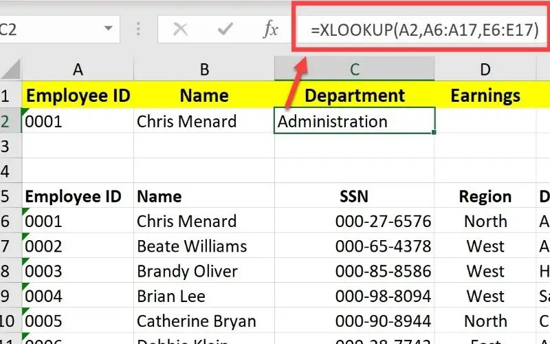
XLOOKUP function is a new function in Microsoft Office 365. This function allows you to look for a dataset’s horizontal or vertical value and then return it to the corresponding value in another row or column. The XLOOKUP function defaults to an exact match and can return multiple results. The formula for using the XLOOKUP function is: =XLOOKUP(lookup_value, lookup_array, return_array, [if_not_found], [match_mode], [search_mode])
9. Unique
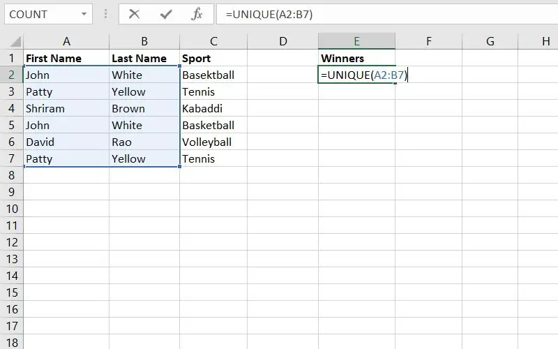
This UNIQUE function is available in Microsoft Office 365. This function will give you a unique list of items in a dataset. This UNIQUE function needs three things:
- Array- Range to get back the unique list, from
- By Col- Whether you would like to check for particular values by column or by row
- Exactly Once- Whether you want a specific or a different list – items that occur only once. The formula for the UNIQUE function is: =UNIQUE(array, by column, exactly once).
10. Offset
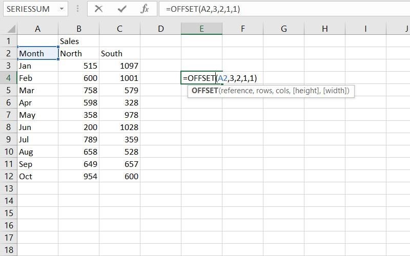
This function is a combination of SUM and AVERAGE. OFFSET is used when you insert continuous rows into an existing database. OFFSET provides a range where you must mention reference cells, the number of rows, and columns. The formula for the OFFSET function is: =OFFSET(reference, rows, column, [height], [width])
