Excel, the renowned spreadsheet software, has revolutionized the way we organize and analyze data. While many individuals may be familiar with basic Excel commands, such as calculating averages and sums, trimming excess spaces, finding minimum and maximum values, counting entries, replacing text, using floor and ceiling functions, performing calculations with exponentiation and power functions, converting negative values to positives, and creating drop-down lists, there exists a realm of more advanced commands that exemplify mastery of this powerful tool. However, the following carefully curated selection of commands, derived from a thorough investigation, possesses the potential to elevate one’s Excel proficiency and establish expertise in the realm of data manipulation.
1. VLookUp
VLOOKUP, short for “Vertical Lookup,” is an Excel function that enables users to search for specific information within a vast dataset.
Standard syntax for VLookUp is “=vlookup(lookup_value, table_array, col_index_num, [range_lookup])”
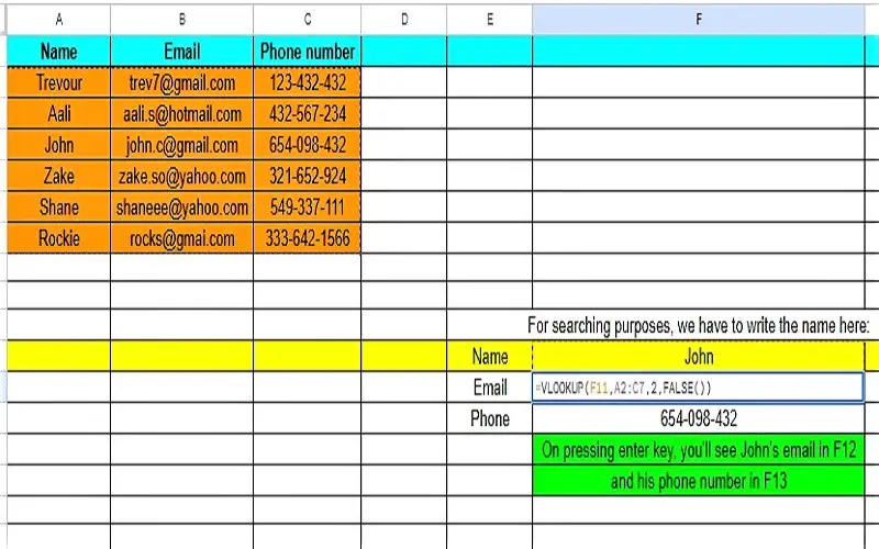
Let’s say you have an Excel sheet with a bulk of data (say starting from A2 and ending at C100), having names (in column 1), email addresses (in column 2), and phone numbers (in column 3).
Now suppose that we have to find John’s email address, so we’d say that:
lookup_value : John
table_array : A2:C100
col_index_num : 2
range_lookup : false (to get an exact match)
2. Concatenation
Concatenate is an Excel function that allows users to combine or join text from multiple cells into a single cell. The process involves:
- Selecting the cells with the desired text
- Specifying any additional text or characters to insert between them
- Using the CONCATENATE function to create the merged result.
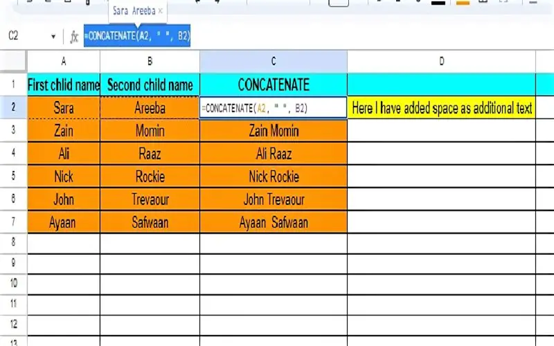
Standard syntax for CONCATENATE “=CONCATENATE(cells you want to merge, “additional optional text”)
We say that we have two cells, i.e., First child name (column 1) and Second child name (column 2). Now, we want to display these names in a single cell, so for that, we’ll use concatenation.
3. IF
The IF function in Excel is a powerful logical function that allows users to perform conditional evaluations and make decisions based on specific criteria.
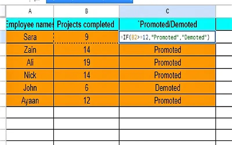
“=IF(condition, output if criterion is TRUE, output if criterion is FALSE)” is the format used for the IF function.
For understanding, let us assume that we have data containing employee names (column 1) and projects completed (column 2). Let the condition in this case be that if the number of projects completed is greater than or equal to 12, then the output should be “Promoted“ otherwise it should display “Demoted“.
4. Remove Duplicates
The “Remove Duplicates” feature in Excel is a built-in tool that eliminates duplicate values from a selected data range, leaving unique data.
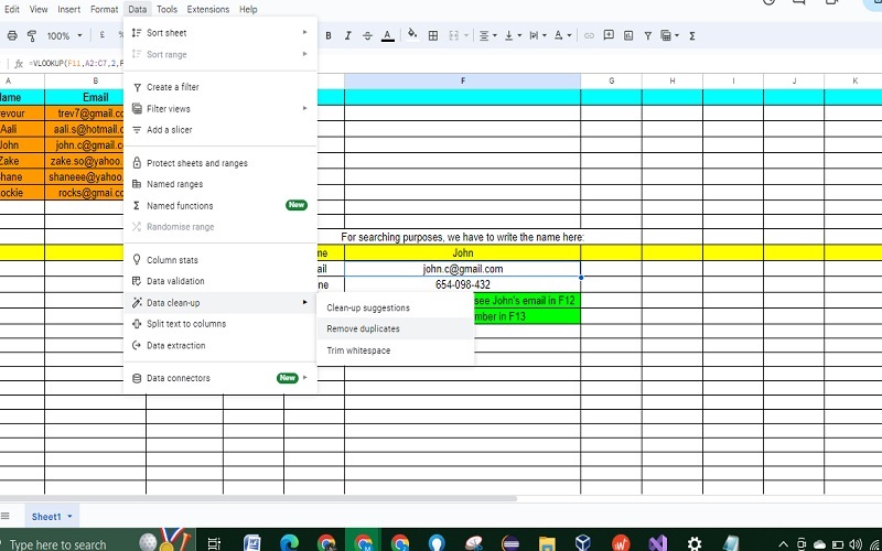
After selecting the data, click Data > Data clean-up > Remove duplicates.
Check the box for the header row if included.
Select cells to remove duplicates with former data (in case you want combination removal from your data). If not, just check the column with the former data.
Click “Remove duplicates“ in the bottom right corner. A new window will display the number of duplicate rows removed and the remaining unique rows.
5. Subtotal
The Subtotal function in Excel is a powerful tool that enables users to calculate various functions, such as sum, average, and count, for specific data groups within a larger dataset.
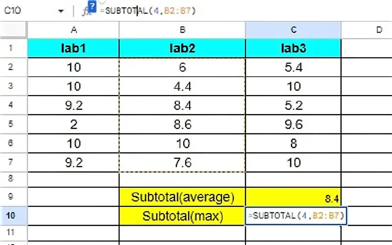
Standard syntax for Subtotal “=SUBTOTAL(func_num, range1, range2)”
Here, func_num can be selected according to the desire; for example, 1 is for average while 4 is for looking up the maximum number in a given range. range1 is compulsory to add (for example A2:A5) where range2 is optional.
6. Index/Match
The INDEX-MATCH combination in Excel is a powerful way to retrieve data from a table based on specific criteria. Instead of using the VLOOKUP function, which has limitations, INDEX-MATCH provides more flexibility.
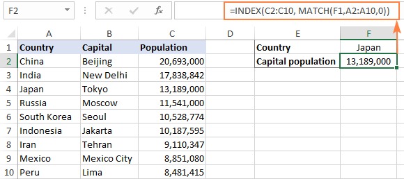
Standard syntax for Index-Match “=INDEX(reference, MATCH(search_key, range, search_type)”
- reference, here you need to enter the data range in which you have to look for the desired data like A2:A17.
- search_key, here you have to enter the data whose corresponding value you are looking for, like J6.
- range is the data where you match the search_key with the lookup array.
- search_type should be set to 0.
7. Countif
The COUNTIF function in Excel is used on a vast scale because of its efficiency. It counts the number of cells according to the given conditions.
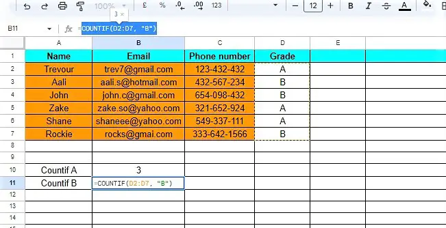
Standard syntax of Countif “=COUNTIF(range, criterion)”
range points to the number of cells that must be counted based on the criteria like A2:A7.
criterion is the criteria in ” ” like “>100” or “A”, etc.
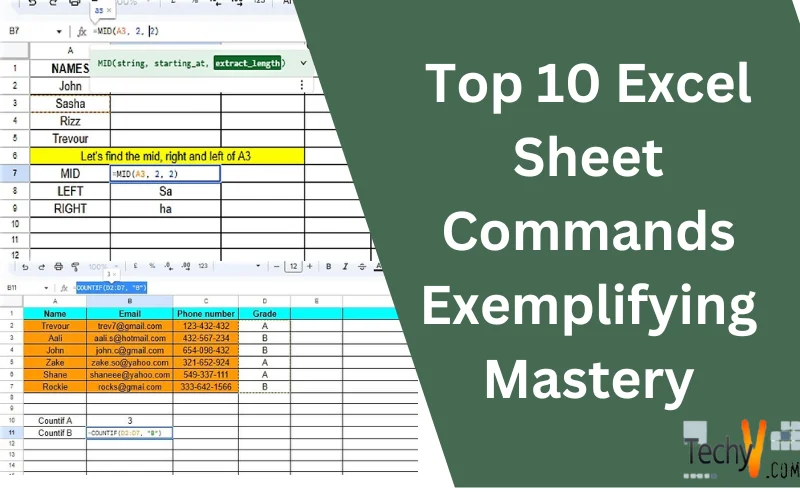
8. Data Extraction Using Left, Right, And Mid Formula
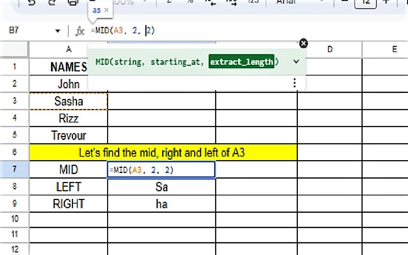
The LEFT, RIGHT, and MID functions in Excel are powerful text functions; used to extract specific portions of text from a cell. LEFT allows users to retrieve characters from the beginning of a cell’s content; RIGHT enables extraction from the end, and MID permits extraction from a specified starting position.
The standard syntax for Left and Right are the same: “LEFT/RIGHT(string, [number_of_characters])”
string is the cell like A2, B6, etc.
number_of_characters is obvious from its name.
Standard syntax for Mid “MID(string, starting_at, extract_length)”
starting_at is the point from where you want to start.
extract_length is the same as number_of_characters
9. Reference
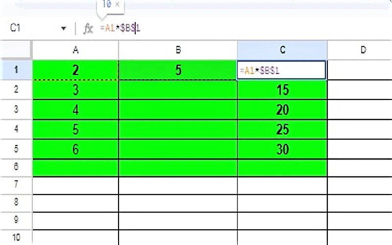
Reference in Excel is a beneficial way to perform calculations on different cells, with one value being a constant available in another cell.
Let’s say we have data from A2 to A17 and B1. Now, we have to multiply A2 to B1 and then A3 to B1 and so on without manually typing it out. Here comes the use of reference. What you have to do is to add the $ sign before every entry of the constant term (in this case, B1, so it will become $B$1).
10. Substitute
The SUBSTITUTE function in Excel allows users to replace specific occurrences of a particular text with a new text within a given cell or a range of cells. It proves beneficial when you want to make selective changes to your data without altering the entire content manually.
Standard syntax for Substitute “=SUBSTITUTE(text_to_search, search_for, replace_with, [occurrence_numnber])”
- text_to_search is the cell name like A2, B3, etc.
- search_for is the text in ” ” that we need to replace.
- replace_with is the new text which we want.
- If the text that is to be replaced occurs more than once then occurrence_number is required.


